
Stage 2 · Annotation
Manual fish annotation: drawing bounding boxes and storing them as queryable relational records.
Abstract
Stage 2 turns the frame dataset from Stage 1 into a supervised-learning dataset in
three steps: the frames are uploaded to Label Studio and every visible fish is boxed
by hand, the labelled project is exported in YOLO format, and each box is parsed into
a relational annotations table keyed back to its source frame. Each labelling batch
is also recorded in an annotation_sets table, together with the sampling and Label
Studio details it came from, so every box stays traceable to its frame, its batch and
its video. The database now holds 4,507 boxes on 837 frames across seven labelling
batches, with no orphaned rows and no coordinates outside the normalised range. This
is the labelled-data layer the detector is trained on in Stage 3.
Introduction
Section titled “Introduction”A detector is only as good as its labels. For AquaMind, the labels are bounding boxes drawn by hand around every visible fish on the frames extracted in Stage 1, and they are a key input to the detector trained in Stage 3.
Labelling tools export these boxes as a folder of text files, one per image. That format is enough to train a model once, but it forgets where the labels came from: which video, which sampling of frames, which labelling session. Here that matters, because frames come from several sources, labels are added in rounds, and a model has to be retrained on chosen subsets. Without that link it is not possible to say which data a given model saw, or to rebuild a dataset later.
Stage 2 therefore treats labels as data with a history. Each box is stored as a record linked to its frame, and each labelling round is recorded as a batch, so datasets are assembled by query instead of by copying folders. This chapter describes how the frames were labelled and stored, and Stage 3 then trains the detector on the result.
Produce a hand-labelled dataset, stored in a relational database, in which every box is traceable to its frame, labelling batch and video, as the source for training the object detector in Stage 3.
Methods
Section titled “Methods”Pipeline overview
Section titled “Pipeline overview”Frames go into Label Studio and come out as YOLO label files, one per frame, each
line describing one bounding box. store_annotations.py combines those files with
sidecar files that record how the batch was built, and writes two MySQL tables: one
that summarises each round of labelling for traceability, and one that holds every
individual bounding box. Fig. 1 shows the full pipeline below.
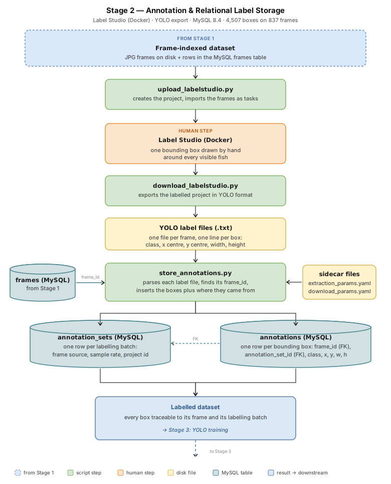
The subsections below follow the pipeline figure from top to bottom: Label Studio is set up first, then each script in turn, with the tables introduced right before the script that first writes to them.
Setting up Label Studio
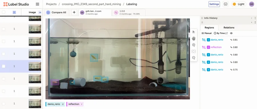
Section titled “Setting up Label Studio”Label Studio runs as a Docker container, so nothing is installed locally beyond Docker
Desktop. A volume mount keeps its data in a local mydata folder on the host, so
labelled work survives a container restart. The upload and download scripts talk to it
through its API, using the address and key stored in the .env file.
Uploading the frames
Section titled “Uploading the frames”upload_labelstudio.py (flow diagram) reads a project name and a frames folder from
config.yaml and creates the project through Label Studio’s API. The labelling interface
is defined in the script and not in the web interface: an image with rectangle labels
for two classes, danio_rerio (hotkey d) and reflection (hotkey r). Reflections
of the fish on the tank glass are a class of their own so that the detector learns to
ignore them, instead of never seeing them. The script then uploads every JPG in the
folder as one task and logs its progress after each upload.
Labelling by hand
Section titled “Labelling by hand”Each task is opened in Label Studio and a bounding box is drawn around every visible fish, one box per fish, plus one for each visible reflection. This is the only manual step in the stage.
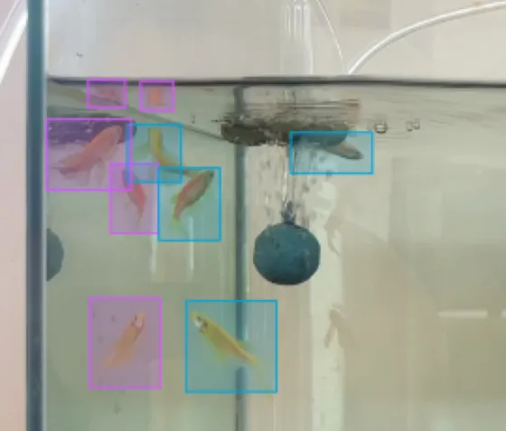
The reflection class is the hard part of the labelling. The glass of the tank acts as a
mirror, so a fish can appear twice in the same frame: once as the animal itself and once
as its reflection. If both were boxed as fish, one individual would be counted twice, and
the detector would be trained to treat a mirror image as a real animal. Boxing reflections
under their own class teaches the model the difference. In the figure below, cyan boxes
mark real fish (danio_rerio) and pink boxes mark reflections (reflection).
The tank adds a second layer of ambiguity. The glass is not the only reflective surface: the water surface also mirrors the scene, so a reflection can itself be reflected again, and a single fish can leave several look-alike images in the same frame. Some of these are faint, distorted or partly cut off, and it is not always obvious where a real fish ends and a mirror image begins. The labelling therefore needs a consistent rule for what counts as a fish and what counts as a reflection, applied the same way on every frame. Otherwise the two classes blur together in the training data. The aim is that a detector trained on these labels learns to tell them apart, but whether it manages this reliably is something the evaluation in Stage 3 has to show, not something the labelling can guarantee.
Exporting in YOLO format
Section titled “Exporting in YOLO format”download_labelstudio.py (flow diagram) looks up the project by name, asks Label Studio for the ids of the tasks that
have been labelled, exports them with
Label Studio’s YOLO export type, and unpacks the archive into a timestamped folder.
Source images can be downloaded as well, but by default they are not, because the
frames already exist on disk from Stage 1. Next to the export the script writes
download_params.yaml, which records the project name and id, the task-id range and
the download time.
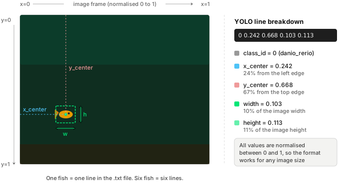
The export contains a classes.txt file with the label names, a labels/ folder with
one .txt file per frame, and a notes.json file with metadata. Each label file has
one line per bounding box, holding five values that are normalised between 0 and 1
relative to the image dimensions, which makes the format independent of resolution.
For example:
class_id x_center y_center width height0 0.242 0.668 0.103 0.113This line is one fish: class 0 (danio_rerio), centred about a quarter of the way
across the frame and two thirds of the way down.
Setting up the tables
Section titled “Setting up the tables”Stage 2 adds two relational tables, both first written to by the script below.
annotations holds one row per bounding box: the frame it sits on (frame_id, a
foreign key into frames), the labelling batch it came from (annotation_set_id, a
foreign key into annotation_sets), the class, and the four normalised box
coordinates. annotation_sets holds one row per labelling batch: the video
(video_id), the frame_source (regular, crossing_event or ghosting_event),
the sampling parameters (sample_rate, start_seconds, end_seconds,
frames_extracted, plus iou_threshold and dedup_window for crossing-event
batches), and the Label Studio project details (name, id, download time and task-id
range).
The batch table was added later in the project, once frames came from more than one
source (see Stage 5), and
annotations gained its annotation_set_id column at the same time. Keeping the
batch details in their own table means they are recorded once per batch, not repeated
on every box, the same split Stage 1 uses for videos and frames.
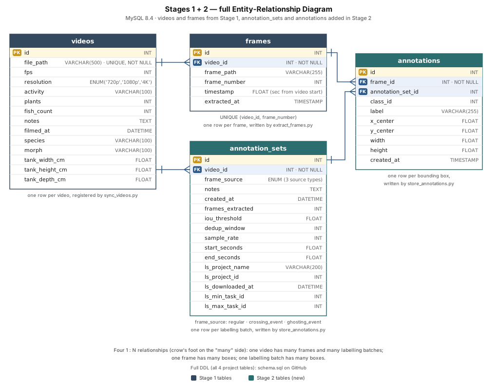
The definitions of all four tables are in
schema.sql
on GitHub.
Storing the annotations
Section titled “Storing the annotations”store_annotations.py (flow diagram) is where the three kinds of input in the pipeline
figure meet: the exported label files, the frames table from Stage 1, and the two
sidecar files. It first reads the sidecars: extraction_params.yaml, written by
Stage 1 when the frames were extracted, and download_params.yaml, written earlier
in this stage by download_labelstudio.py. From the two combined, plus the video name in config.yaml (used to look up the
video’s id), it creates one annotation_sets row for the batch, which gives it a batch id. It then loops over
the .txt files in labels/, one per frame.
Label Studio prefixes each exported file with a hash (for example
e6d83681-frame_360.txt), so the script parses the frame number out of the file name
and looks it up in the frames table to get the frame_id. The lookup matches on
both the frames folder and the frame number, because the same frame number can occur
in different extraction runs of the same video. A frame that is not in the table is
skipped with a warning, so a label can never be stored against a missing frame.
Each line in a label file is one box. The five values are cast (class_id to int,
the four coordinates to float), a line with fewer than five values is skipped
with a warning, and the class id is mapped to its name. Every box is inserted into
annotations with its frame_id and the batch id, and a single commit at the end
saves the whole batch, so a run that fails partway saves nothing. The script finishes
by printing the batch id and a ready-made SQL query for counting the boxes in it.
Results
Section titled “Results”Correctness was verified by querying the tables directly (counts as of 2026-09-21). Seven labelling batches are stored, from three kinds of frame source:
| Annotation set | Frame source | Frames with boxes | Bounding boxes |
|---|---|---|---|
| 5 | regular | 46 | 445 |
| 8 | crossing_event | 121 | 781 |
| 9 | regular | 103 | 719 |
| 10 | regular | 111 | 224 |
| 11 | crossing_event | 73 | 355 |
| 14 | crossing_event | 109 | 598 |
| 17 | ghosting_event | 274 | 1385 |
| Total | 837 | 4,507 |
Frames that were uploaded but ended up with no stored box do not appear in
annotations, so the frame counts here are frames that hold at least one box.
Beyond the counts, the stored boxes were checked for a missing batch link and for
coordinates outside the normalised range. A missing frame link is ruled out by the
foreign key on frame_id. The class balance and the boxes per frame were read off the
same tables:
| Check | Result |
|---|---|
| Boxes without a labelling batch | 0 |
| Boxes outside the normalised range | 0 |
| Boxes per class | 3,600 danio_rerio, 907 reflection |
| Boxes per frame | 5.4 on average, 26 at most |
Discussion
Section titled “Discussion”Stage 2 turns hand-drawn boxes into a queryable dataset. Each box is a row linked to its frame and to the labelling batch it came from, and each batch is linked to its video, so a question such as which frames of which video a model was trained on has a SQL answer. Keeping the batches in their own table is what lets Stage 3 pick a training set by listing batch ids, and it is what makes each model version traceable to the data it saw.
Two design choices are worth stating. Reflections are labelled as their own class instead of being left unlabelled, so the detector is shown what to ignore. And the frame lookup checks the frames folder as well as the frame number, so labels from different extraction runs cannot be attached to the wrong frame.
The main limit is that the labelling is manual and was done by a single annotator, so there is no measure of labelling agreement. The frames also come from one tank and a small group of fish. Later rounds reduce the manual cost in two ways, described in Stage 5: the trained detector pre-labels new frames so they only need correcting, and the frames worth labelling are chosen from the tracker’s failures. The labelled dataset feeds Stage 3, where the detector is trained.