
Stage 8 · Feeding-strike detection
Feeding-strike detection: classical and deep learning both fail, a simple burst signal still helps
Abstract
A feeding strike is a fast, subtle appearance-and-posture event with no visible
prey to anchor on, which makes it a harder computer-vision target than the
spatially “loud” behaviours of earlier stages. This stage tests whether a strike
can be detected automatically from video, and how far a geometry-only approach
gets before appearance information is needed. A geometry-only baseline (logistic
regression, random forest, XGBoost on the same four kinematic features) lands
at or below chance across all three classifiers (0.56 / 0.54 / 0.49
accuracy), which is the evidence that appearance features are actually
required. A CNN-LSTM on image crops (DINOv2 vits14 features into an
LSTM, with early stopping) reaches 64 % accuracy, 0.66 precision, 0.68 recall
on a balanced test split, but a negative control run over a realistic, continuous
stream shows that result does not hold: the model calls a strike on 46 % of
ordinary-swimming windows versus 64 % of real-feeding windows, close to
indistinguishable from chance. Both approaches land as a benchmarked negative
result: the strike-defining cues are not resolvable from centroid tracks or
re-ID-oriented crops at this frame rate, a data limitation rather than a
fixable modelling gap. A third, deliberately simpler approach then recovers a
usable signal from the same tracked data: a group-level burst-rate index,
built from nothing more than smoothed speed peaks against a control-only,
data-derived threshold, rises from a control mean of 2.94 to a feeding
mean of 4.17 events/sec, a roughly 1.4x increase, and tracks real feeding
closely enough on direct visual inspection to work as a lab-condition readout
where both purpose-built classifiers could not.
Introduction
Section titled “Introduction”A feeding strike is the fast lunge and capture a fish makes when it takes prey. Behavioural ecology treats it as one of the single most informative behavioural cues, especially in larval fish, because a trained observer can read from it the factors acting on the animal. It is also very subtle and hard to score by eye, and automated detection is not established for fish at any real scale in ecology. A detector that worked would be valuable, and in the long run could support routine scoring in the lab.
For computer vision, a feeding strike is a harder target than the behaviours in the previous stage. Chasing, depth preference and other spatially “loud” behaviours have a clear geometric signature: they are defined by where a fish is and how it moves relative to the tank or to another fish. A feeding strike is not. Its signal lives in appearance and posture (a brief body vibration or S-bend and a mouth gape) rather than in position. The prey is a tiny particle, invisible at screen resolution, so there is no visible target to anchor on. The whole event is short and easy to miss when the fish is not in sharp focus.
This stage tests whether a feeding strike can be detected automatically from video, and how far a geometry-only approach gets before appearance information is needed. The one component that might still carry a geometric signal is the burst, since a strike burst may be faster or sharper than one in normal swimming. Even so, I expect it will not be enough on its own, and that reliable detection needs a model working from the image directly: a CNN extracting appearance and posture per frame, a sequence model learning how they change across the strike. The stage is built in that order: a geometry-only baseline first, then a CNN-LSTM pipeline on image crops.
Methods
Section titled “Methods”Stage 8 trains a per-fish feeding-strike classifier from a set of hand-labelled strike events. Two approaches are compared on an identical set of windows: a geometry baseline built from movement alone, and a CNN-LSTM built from the fish’s appearance. The appearance model is the one of interest, because a feeding strike has little geometric signature, and the baseline is there to test that rather than assume it. Fig 1 shows the pipeline end to end; the subsections below follow it in order, and each step is a single script whose output file is the next step’s input.
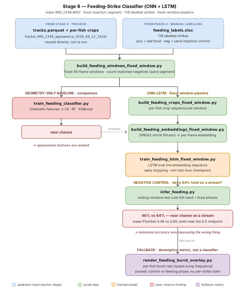
The feeding-experiment recording (IMG_2349.MOV; watch the tracked recording ↗) is
already tracked from earlier stages, so tracks.parquet and the per-fish crops are reused
directly. It has three phases of about two minutes each: a calm baseline, a
control-injection phase in which tiny sand particles are delivered through the
same tubing later used for the food (frames 7505 to 14340), and a food-injection
phase (from frame 14340). 118 real strikes were labelled by hand, all of them
in the food-injection phase (frames 14617 to 21656).
Positives are taken from the food phase and negatives from the control-injection phase, not from the calm baseline. Both phases involve an injection through the tubing and the fish reacting to it, so the main systematic difference between a positive and a negative window is whether food was present; calm-baseline negatives would instead let the model succeed by detecting disturbance rather than feeding. The match is approximate, since injected sand settles within seconds while a feeding bout keeps the fish foraging for longer, but it is a closer control than calm footage. The chaotic feeding-frenzy burst right at the food-injection point is excluded from both classes: occlusion and ID-switch risk there make reliable per-fish attribution unsafe.
Window construction
Section titled “Window construction”build_feeding_windows_fixed_window.py turns each labelled strike into a
fixed-length window centred on the midpoint of its labelled frame range, the
frame where the strike itself is visually clearest. A feeding strike, as
labelled by eye, is an extremely subtle event: a brief shake or vibration of
the body, sometimes with the mouth visibly opening, and it is frequently
accompanied by a change of swimming direction right at the strike, as the
fish turns onto the food. Any one of these three cues (the shake, the mouth,
the turn) can be the clearest signal in a given case, and none of them is
reliably visible in every strike, which is part of why the window is centred
on the labeller’s best estimate of that moment rather than on a single
detectable trigger. A fixed length is used rather than each event’s real span
because a deployed detector sees
a continuous stream with no event boundaries: a fixed window slides along the
input directly, while an event-length window would first need a separate stage to
locate candidate events. The length is set to 45 frames (0.75 s at 60 fps), the
75th percentile of labelled strike duration, so most windows contain the whole
strike and the rest still contain its central lunge; a longer window was avoided
because strikes occur roughly once a second during the feeding bout, so it would
often capture a second strike. For each positive window the script draws one
non-overlapping negative window at random from the control-injection phase,
assigned to a random fish. Any window holding a frame the
tracker flagged as occluded or missing is dropped, so both approaches train and
test on exactly the same windows. The script then makes a label-stratified 80/20 train/test split,
before any crops or features exist; because there is one non-overlapping window
per event, no frame from a test strike reaches training. Its output, train_df
and test_df (one row per window: fish id, frame range, label, split), is the
single source of truth for window membership everywhere downstream.
Approach 1 — Geometry baseline
Section titled “Approach 1 — Geometry baseline”Speed and burst are used here because they are the only strike cues that survive centroid tracking at all. Of the three visual cues described above, the body shake is a genuine movement event and so has some chance of showing up in a speed trace; the mouth gape does not; the fish is filmed side-on in a whole-tank shot, and a strike can happen facing away from or across the camera as easily as toward it, so the mouth is frequently too small on screen or hidden by the fish’s own body and orientation to be usable as a tracked geometric feature at all, even before considering resolution. The direction change is closer to a heading feature than a speed one, and is not included in this baseline; it is the natural next feature to add if this approach is revisited (see Discussion).
train_feeding_classifier.py reads the window tables and computes four kinematic
features per window: mean and maximum speed, and mean and maximum burst, where
burst is the frame-to-frame change in speed. Speed is capped at the 99.9th
percentile and smoothed with a 5-frame centred rolling mean before burst is
derived, to suppress single-frame tracker-jitter spikes. The four features feed
three standard classifiers, logistic regression, a random forest and XGBoost,
left at their library defaults with no hyperparameter tuning and compared
directly: if a real boundary existed in these features, a plain off-the-shelf
model should be enough to find it, so a null result here is not explained
away by “the wrong algorithm.” Mean and maximum speed, mean and maximum burst
are the
most direct kinematic quantities a fish’s tracked position can give: the
first pair asks how fast it moved, the second how sharply that speed changed,
and between them they are the natural first features to try before reaching
for anything more elaborate.
Approach 2 — Appearance model (CNN-LSTM)
Section titled “Approach 2 — Appearance model (CNN-LSTM)”The appearance path is three scripts. build_feeding_crops_fixed_window.py
expands each window into 45 ordered per-frame rows, each pointing at that frame’s
crop image (the tracker already saved the crops; this only builds the manifest),
written grouped by event. build_feeding_embeddings_fixed_window.py loads a
frozen DINOv2 vits14 backbone once and passes each window’s 45 crops through it
in frame order, producing a (45, 384) embedding sequence; because the backbone
never trains, these are computed once and cached as .pt files rather than
recomputed each epoch. train_feeding_lstm_fixed_window.py then trains the only
part that learns: a single-layer LSTM (hidden size 64) that reads the embedding
sequence, with a linear head mapping its final hidden state to strike or no
strike. Training uses cross-entropy with Adam (learning rate 1e-3, batch size 8)
for up to 100 epochs.
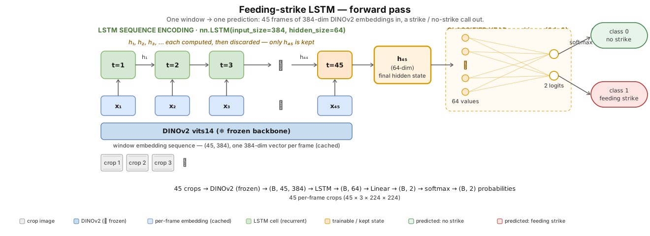
At training time, this forward pass runs once per window inside each batch of 8, followed by cross-entropy loss and a backward pass (Adam, lr=1e-3), repeated for up to 100 epochs, keeping the checkpoint at minimum test loss. At inference time, the identical forward pass runs once per window, with no labels and nothing after it but recording the score; sliding across a continuous video is a separate, outer loop wrapped around this same computation, not a different model.
Inference and evaluation
Section titled “Inference and evaluation”Both models are first scored on the same held-out 20 percent test split, which is untouched during feature smoothing, training and checkpoint selection. Accuracy, precision and recall are reported for the strike class, where a false positive is a window predicted as a strike that was not one. For the CNN-LSTM, training and test loss are logged every epoch and the curves are read directly rather than trusting the final-epoch score, since on a dataset this small the training loss can keep falling well after the test loss has bottomed out; the model kept for reporting is the checkpoint at minimum test loss, not the last epoch.
A separate script, infer_feeding.py, evaluates the trained CNN-LSTM a second way. Rather
than scoring a fixed, curated set of windows, it runs the same forward pass
shown in Fig 2 as a sliding-window classifier directly over two full segments
of the same recording, the sand-injection phase and the food-injection phase,
stepping a 45-frame window forward 20 frames at a time so consecutive windows
overlap. Any window missing a tracked crop anywhere in its 45 frames is
dropped; every window that survives is scored independently, with no labels,
no train/test split and no backpropagation involved, since the model is
already trained and frozen at this point. This is a direct test of whether the
balanced-split numbers above hold up once the model is run the way it would
actually be used: continuously, on ordinary swimming as well as real feeding,
rather than on a hand-picked 50/50 set.
Approach 3 — Burst-rate (group-level fallback)
Section titled “Approach 3 — Burst-rate (group-level fallback)”Once Approaches 1 and 2 both failed the stream test above, render_feeding_burst_overlay.py
drops per-fish, per-strike attribution entirely. It reuses the same
tracks.parquet and per-fish speed (smoothed the same way as the geometry
baseline) to detect bursts as local peaks in speed via scipy.signal.find_peaks,
then pools burst counts across all fish rather than assigning any burst to a
specific strike or fish. Bursts are compared as a rate (events per second)
across two segments of the same recording: control (calm baseline plus the
sand-injection phase, collapsed together since both are “no real food”) and
real feeding. This is a deliberately smaller claim than either classifier
above: it asks only whether the group’s overall burst rate shifts with real
feeding, not which fish struck or when.
A speed peak only counts as a burst if it clears three gates, all applied in
one find_peaks call:
- height ≥
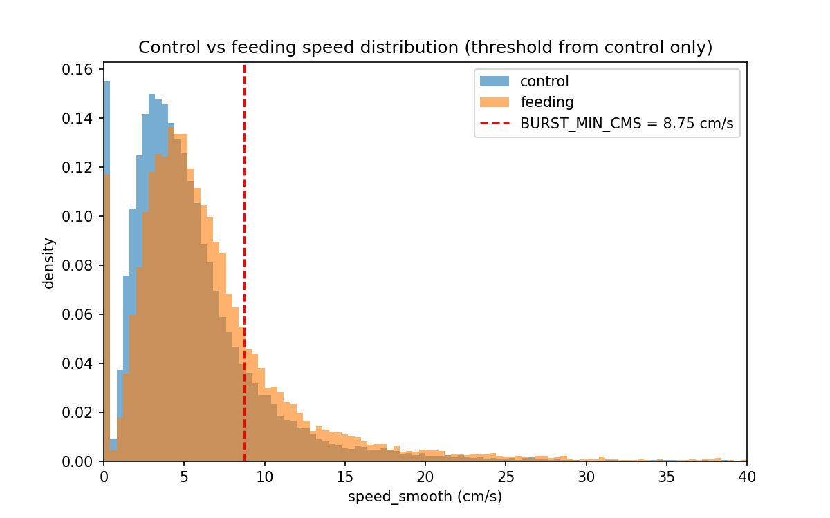
BURST_MIN_CMS, the 85th percentile of smoothed speed measured during the control segment alone, with the feeding segment excluded from that calculation so the effect under study cannot leak into the baseline used to detect it (data-derived rather than picked by eye, landing at roughly 8.75 cm/s here) - prominence ≥ 4.0 cm/s, so the peak has to stand out from its own local dip, not just ride along the top of an already-elevated stretch
- distance ≥ 0.4s between peaks, so two spikes closer together than that count as one burst rather than the same lunge counted twice
Results
Section titled “Results”Three approaches were tested, in the order the stage was built: a geometry-only baseline, the CNN-LSTM appearance model, and, once neither survived a realistic stream test, a purely descriptive burst-rate fallback. Each is reported here as its own approach, with its own numbers.
Approach 1 — Geometry baseline
Section titled “Approach 1 — Geometry baseline”All three classifiers are trained on the same four kinematic features (mean speed, maximum speed, mean burst, maximum burst), scored on the strike class, on the same held-out 20 percent test split used for every model in this stage (balanced roughly 50/50 between labelled strikes and matched negatives). Reported separately rather than as one collapsed number, since the point is whether any classifier can find a usable boundary in these features, not which one happens to win:
| Model | Accuracy | Precision (feeding) | Recall (feeding) |
|---|---|---|---|
| Logistic regression | 0.56 | 0.55 | 0.80 |
| Random forest | 0.54 | 0.54 | 0.70 |
| XGBoost | 0.49 | 0.50 | 0.45 |
All three sit at or below chance-equivalent for a balanced binary split, with XGBoost landing exactly at coin-flip accuracy. Logistic regression’s higher recall alongside near-chance precision is a further sign of a weak, mostly linear nudge rather than a real decision boundary: the model is closer to calling “feeding” more often than to actually separating the classes. This is the expected result, not a failure: it is the evidence that a feeding strike has too little geometric signature for movement alone, and that appearance information is needed.
Approach 2 — CNN-LSTM (appearance)
Section titled “Approach 2 — CNN-LSTM (appearance)”| Model | Accuracy | Precision | Recall |
|---|---|---|---|
| CNN-LSTM, fixed 45-frame window | ~0.64 | 0.66 | 0.68 |
On the balanced test split the CNN-LSTM looks like it might be a working detector. It is not one.
A negative control makes this concrete. infer_feeding.py runs the trained model as a
sliding-window classifier over two full segments of the same recording: the
sand-injection phase, where no food is present and the correct strike count is
zero for every fish, and the food-injection phase, where real feeding happens.
| Segment | Positive windows | Rate | Mean P(strike) |
|---|---|---|---|
| No food (sand-injection phase) | 497 / 1080 | 46.0% | 0.476 |
| Real feeding | 587 / 917 | 64.0% | 0.598 |
The model calls a strike on nearly half the windows drawn from ordinary swimming with no food present, against a true count of zero, and on 64 percent of windows during real feeding, only 18 points higher. The 64 percent balanced-split accuracy figure is real; it was measured on the wrong population.
The LSTM’s own decision-threshold sweep, recorded before the negative control was ever run, already carried a warning. Raising the classification threshold from 0.5 to 0.6 to 0.7 made precision, recall and accuracy all worse at once, with 0.5 winning outright. A model with real class separation trades recall for precision as the threshold rises, keeping only its most confident calls; this one had no such structure to isolate, because its output probabilities were never meaningfully separated in the first place, the same fact the stream test later confirmed directly (0.476 vs 0.598, both close to the 0.5 midpoint).
Approach 3 — Burst-rate (group-level fallback)
Section titled “Approach 3 — Burst-rate (group-level fallback)”Neither the geometry baseline nor the CNN-LSTM survives a realistic stream, so
the last approach drops per-fish, per-strike attribution altogether and asks a
smaller, honest question instead: does a fish’s burst rate change between
control and feeding at the group level? render_feeding_burst_overlay.py counts speed
peaks (bursts) per fish from the same tracked recording, pooled across all
fish, with no attempt to say which fish struck or when.
| Segment | Pooled burst rate (events/sec) |
|---|---|
| Control (baseline + sand injection) | 2.94 |
| Real feeding | 4.17 |
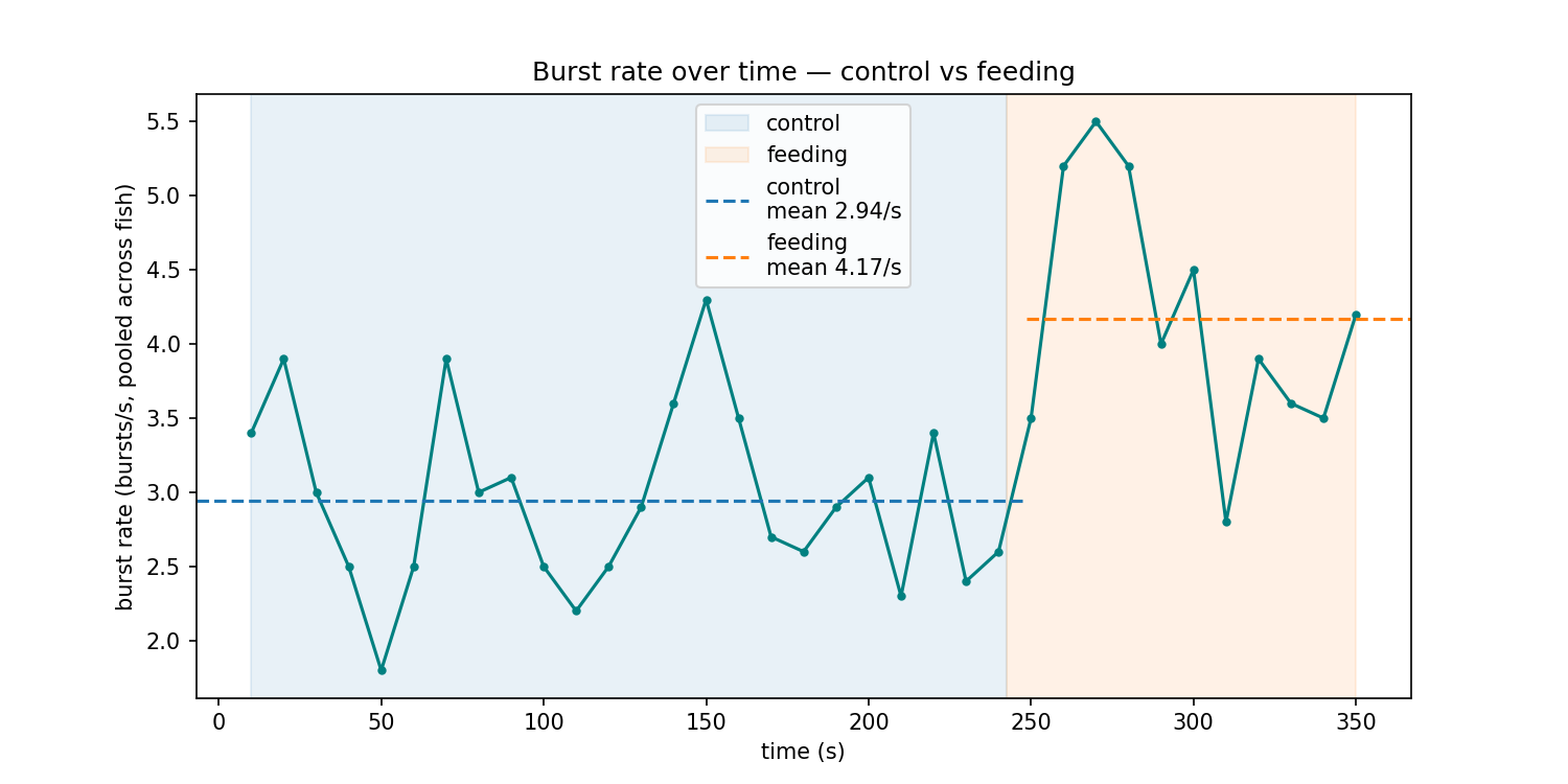
Burst rate rises roughly 1.4x from control to real feeding. It does not need to solve the per-strike attribution problem the previous two tests failed at, since it never claims to say which fish struck or when; it is a legitimate before/after readout for the alarm-cue assay, and the closest thing to a working deliverable this stage produced.
Discussion
Section titled “Discussion”A model that flags a strike on nearly half of all ordinary swimming is not a slightly-off detector. It is not a detector at all, and that is the real headline of this stage, not the 64 percent balanced-accuracy score that looked like a working result until it met a realistic stream instead of a curated 50/50 split. The same trained model called a strike on 46 percent of ordinary-swimming windows, true count zero, barely below its 64 percent hit rate on windows that actually held one. A number that confident and that wrong is not a tuning problem, it traces to what the data can carry, not to the model or the pipeline. A zebrafish strike is defined by a mouth gape and eye convergence, at a scale specialist studies (Shamur et al. 2016, filming at 240 fps with head-orientation normalisation) still cap around 73 percent accuracy for. At 60 fps, whole-tank, working from centroid tracks and re-ID-oriented crops, neither cue is resolvable, confirmed directly on a labelled clip where the fish’s centroid barely moves during a strike, since the event is a head snap rather than a translation.
Studies that do recover gape and posture at this level of detail, such as Mearns et al. (2020), classify capture bouts from tail-posture and timing-to-max-gape measurements extracted at a level of kinematic detail this whole-tank, 60 fps setup was never built to capture. The plausible mechanism is that a strike this brief and this small on screen leaves little trace once compressed into a bounding-box crop and an embedding, though this pipeline did not isolate that mechanism directly, only its consequence. More labelled data would not fix it either way: both approaches failed from a ceiling on what the features themselves carry, not from too few examples, so what would actually help is different data, a higher frame rate and a jaw or head keypoint, not more labels from the same recording. Phase G (an overlay, per-fish counters, an automated report) is dropped accordingly; there is nothing trustworthy to visualise from either classifier, and the chasing classifier from the previous stage remains this project’s working behaviour detector.
The clearest surprise of this stage sits outside the classifiers entirely. Watching the burst-rate index (Approach 3) directly against the video by eye, it tracks real feeding closely: minutes with visibly more fast movement are, on inspection, minutes where fish are actually striking, closer than either learned model ever managed on its own test split. The likely reason is the same failure seen from the other side. The CNN-LSTM was asked to learn a cue that is not present in its inputs at this resolution, so its output probabilities sit near 0.5 and flicker close to at random, while peak detection on smoothed speed asks a much smaller, answerable question, not “is this fish gaping at prey” but “is this fish moving unusually fast right now.” Complexity did not help here because the extra capacity had nothing extra to learn from, and the simplest tool in the stage ended up reading the behaviour best.
The match is not unconditional: as food is consumed and becomes scarce, bursts blend back into ordinary locomotor activity and can no longer be told apart from a fast turn on their own. Read that decline as a feature rather than a flaw and the metric is doing something biologically sensible, tracking perceived prey availability rather than strikes directly, which is exactly the behaviour a foraging fish should show as a patch depletes. What survives for measurement is the trend around a known injection point, not the individual event, a strong lab-condition tool rather than a general in-vivo one. That trend is still only as trustworthy as the cutoff used to call a speed peak a burst in the first place, and the control and feeding distributions overlap enough that no single frame gives away which condition it came from; somewhere past their shared peak, in the population of frames rare rather than typical, the two curves finally pull apart.
The threshold used here is the 85th percentile of speed from the calm-baseline-plus-sand segment, with the food-injection segment excluded from that calculation on purpose. The exclusion matters more than the percentile: fold feeding speeds into the same calculation and a real speed increase from feeding raises the very bar feeding then has to clear, so a strong effect would make itself harder to see, not easier. Someone has already tried removing that kind of arbitrariness altogether. Wang, Kroeschell, Zhu, Mumm and Yi (bioRxiv, 2026) train a CNN-BiLSTM on hand labelled tail kinematics to detect swim bouts in tethered larval zebrafish with no cutoff at all. Their own numbers mark where that effort earns its keep: on high-amplitude bouts the learned model ties a plain threshold, 97.7 against 98.0 percent accuracy, and only pulls ahead on subtle, low-amplitude events, where precision climbs from 67 to 89 percent. A feeding-driven burst is the large, high-amplitude case their results already call solved without a model, which is why a percentile threshold, not a learned one, was kept here.
What that threshold cannot do yet is travel. Run this same calibration on a different day, tank, or the same fish a month later, and each one quietly recomputes its own cutoff, blind to every other session, so a genuine rise in baseline activity across a study would vanish into a moving target rather than showing up against a fixed one. The fix costs nothing extra: pool control-segment speed across every session or tank first, take the percentile once, and hold it fixed for the rest of the study, a number that means the same thing on day one and day thirty, tank A and tank B, before anyone outside a single recording has reason to trust it. That is the natural next step for per-strike detection too, treated as still open rather than closed: a movement-based feature set richer than raw speed, closer to the bearing and lagged path-following features already scoped for the chasing classifier in Stage 7, combined with the burst signal and its pooled threshold, is a more promising direction than a bigger appearance model on the same crops. None of that is built or claimed here; it is the concrete direction this negative result points toward, needing considerably more labelled sessions and cross-tank testing before any of it could be trusted.
References
Section titled “References”Shamur, E., Zilka, M., Hassner, T., China, V., Liberzon, A., & Holzman, R. (2016). Automated detection of feeding strikes by larval fish using continuous high-speed digital video: a novel method to extract quantitative data from fast, sparse kinematic events. Journal of Experimental Biology, 219(11), 1608-1617.
Wang, H., Kroeschell, G., Zhu, Y., Mumm, J. S., & Yi, J. (2026). Threshold-free neural network models for swim bout detection of larval zebrafish. bioRxiv.
Mearns, D. S., Donovan, J. C., Fernandes, A. M., Semmelhack, J. L., & Baier, H. (2020). Deconstructing hunting behavior reveals a tightly coupled stimulus-response loop. Current Biology, 30(1), 54-69.